Here we will consider sampling a normal distribution   $n$   mutually independent times, and consider the density function for mean of the sample.   That is, let   $X$   be a normal random variable with density function   ${\displaystyle Z_{\mu ,\sigma }}$ , and let   ${\displaystyle X_1}$ , ${\displaystyle X_2}$ , … , ${\displaystyle X_n}$   be   $n$   mutually independent samples of   $X$ .   Then
$$\overline{X}=\frac{1}{n}(X_1+\cdots +X_n)$$
will be the random variable denoting the mean of the sample.

For the purposes of determining the density function of   $\overline{X}$ , we will first determine its moment generating function.

We already know how to compute the moment generating function for a linear combination of independent random variables.   That is, we have seen that if   ${\displaystyle X_1}$ , … , ${\displaystyle X_n}$   are mutually independent, then
$$M_{a_1{X}_1+\cdots +a_n{X}_n}(t)=M_{a_1{X}_1}(t)\cdot M_{a_2{X}_2}(t)\cdot \cdots \cdot M_{a_n{X}_n}(t)=M_{X_1}(a_{1}t)\cdot M_{X_3}(a_{2}t)\cdot \cdots \cdot M_{X_n}(a_{n}t)\text{.}$$
Thus
$$M_{\overline{X}}(t)=M_{\frac{1}{n}{X}_1}(t)\cdot M_{\frac{1}{n}{X}_2}(t)\cdot \cdots \cdot M_{\frac{1}{n}{X}_n}(t)=M_{X_1}\left(\frac{t}{n}\right)\cdot M_{X_2}\left(\frac{t}{n}\right)\cdot \cdots \cdot M_{X_n}\left(\frac{t}{n}\right)\text{.}$$
Since the random variables   ${\displaystyle X_1}$ , … , ${\displaystyle X_n}$   all share the same density function, this gives
$$M_{\overline{X}}(t)=M_X{\left(\frac{t}{n}\right)}^n\text{.}$$

We have already determined the moment generating function for the normal random variable   $X$   with density   ${\displaystyle Z_{\mu ,\sigma }}$   to be
$$M_X(t)={\mathrm{e}}^{\mu t+\frac{1}{2}{\sigma }^2{t}^2}\text{.}$$
This allows us to say that
$$M_{\overline{X}}(t)={\left({\mathrm{e}}^{\mu \frac{t}{n}+\frac{1}{2}{\sigma }^2{\left(\frac{t}{n}\right)}^2}\right)}^n={\mathrm{e}}^{\mu t+\frac{1}{2}\left(\frac{{\sigma }^2}{n}\right)t^2}\text{.}$$

The special thing about this is that the resulting moment generating function looks a lot like that of   ${\displaystyle Z_{\mu ,\sigma }}$ .   In fact, it is precisely the moment generating function of   ${\displaystyle Z_{\mu ,\frac{\sigma }{\sqrt{n}}}}$ .   We have already noted that the moment generating function for a random variable completely determines the probability density function of that random variable.   Consequently   $\overline{X}$   has density   ${\displaystyle Z_{\mu ,\frac{\sigma }{\sqrt{n}}}}$ .   That is, $\overline{X}$   is also a normal random variable, with the same mean as   $X$ , but a smaller standard deviation   –   i.e.   ${\displaystyle \frac{\sigma }{\sqrt{n}}}$   rather than   $\sigma$ .

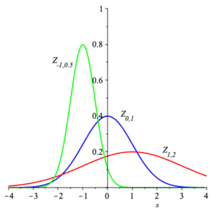
Here are graphs of the density functions for   ${\displaystyle Z_{1,2}}$ , ${\displaystyle Z_{0,1}}$ , and   ${\displaystyle Z_{-1,\frac{1}{2}}}$ .   Notice how the density function with smaller standard deviation has graph much more concentrated about the mean.

The above observation regarding the average of a sample from a normal random variable can be seen as a generalization of an easier fact.

Sum of Independent Normal Random Variables

Fact:   Let   ${\displaystyle X_1}$   and   ${\displaystyle X_2}$   be two independent random variables, with means   ${\displaystyle {\mu }_1}$   and   ${\displaystyle {\mu }_2}$ , and variances   ${\displaystyle {\sigma }_1^2}$   and   ${\displaystyle {\sigma }_2^2}$ , respectively.   Then
$$X_1+X_2$$
is a normal random variable, with mean   ${\displaystyle {\mu }_1+{\mu }_2}$   and variance   ${\displaystyle {\sigma }_1^2+{\sigma }_2^2}$ .

This can be seen by following the logic above.   The moment generating functions for   ${\displaystyle X_1}$   and   ${\displaystyle X_2}$   are
$$M_{X_1}={\mathrm{e}}^{{\mu }_{1}t+\frac{1}{2}{\sigma }_1^2{t}^2}\text{and}{M}_{X_2}={\mathrm{e}}^{{\mu }_{2}t+\frac{1}{2}{\sigma }_2^2{t}^2}\text{,}$$
respectively.   Thus
$$\begin{array}{rl}{M}_{X_1+X_2}& =M_{X_1}{M}_{X_2}\\ & \\ & ={\mathrm{e}}^{{\mu }_{1}t+\frac{1}{2}{\sigma }_1^2{t}^2}{\mathrm{e}}^{{\mu }_{2}t+\frac{1}{2}{\sigma }_2^2{t}^2}\\ & \\ & ={\mathrm{e}}^{({\mu }_1+{\mu }_2)t+\frac{1}{2}({\sigma }_1^2+{\sigma }_2^2)t^2}\end{array}$$
is the moment generating function for ${\displaystyle Z_{{\mu }_1+{\mu }_2,\sqrt{{\sigma }_1^2+{\sigma }_2^2}}}$ .   That is, ${\displaystyle X_1+X_2}$   is a normal random variable with mean   ${\displaystyle {\mu }_1+{\mu }_2}$   and variance   ${\displaystyle {\sigma }_1^2+{\sigma }_2^2}$ .

Here are a couple of computational examples.

Example: A standard normal random variable, $X$   (with density   ${\displaystyle Z_{0,1}}$ ), takes values in the interval   $[-1.96,1.96]$ , symmetric about its mean, with   $95\mathrm{\%}$   probability.   If   $\overline{X}$   is the sample mean of twenty-five samples of   $X$ , find the interval symmetric about its mean within which   $\overline{X}$   takes   $95\mathrm{\%}$   of its values.

Since   $X$   and   $\overline{X}$   both have the same mean, ${\displaystyle {\mu }_X={\mu }_{\overline{X}}=0}$ , $\overline{X}$   has density function   ${\displaystyle Z_{0,\frac{1}{\sqrt{25}}}=Z_{0,0.2}}$ .   This takes   $95\mathrm{\%}$   of its values in the symmetric interval   $[-\frac{1.96}{5},\frac{1.96}{5}]=[-.392,.392]$ .

Example: If   $X$   is standard normal random variable, how large must a sample be to ensure that   $\overline{X}$   takes   $95\mathrm{\%}$   of its values in   $[-.15,.15]$ ?