Many situations of interest are modeled not by normal random variables, but by others that are non particularly close to normal. We have seen examples where it makes sense to use Bernoulli, or geometric, or Poisson random variables. These are discrete, and their densities look nothing like those of normal random variables. But it is a remarkable fact that even in these cases, for sufficiently large values of $n$ we have that $\bar{X}_n$ is well approximated by normal distributions. Moreover, this fact does not depend on the random variable $X$ with which we start. All that matters is that $X$ have a mean $\mu$ and a variance $\sigma^2\;$ . That is, if random variable $X$ has a mean $\mu$ and a variance $\sigma^2\,$ , then as $n\to\infty$ the distribution of $\bar{X}_n$ tends toward a normal distribution. This is a powerful fact, and allows for many important applications. It turns out to be so important that it is given a special, rather high-falutin’ name.
Central Limit Theorem: (CLT) Let $X$ be a random variable having mean $\mu$ and a variance $\sigma^2\;$ . Consider the random variable
$$ Y_n =\frac{\bar{X}_n -\mu}{\frac{\sigma}{\sqrt{n}}} \;\text{.} $$
As $n\to\infty\,$ , the distribution function of $Y_n$ approaches the standard normal distribution function $Z_{0,1}\;$ . This is to be interpreted as saying that (for any $a, b\in\mathbb{R}\,$ ) the probability of $\displaystyle{ Y_n }$ takes on values between $a$ and $b$ becomes ever closer to the probability that $\displaystyle{ Z_{0,1} }$ takes on values between $a$ and $b\;$ .
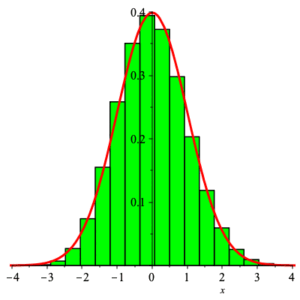
Here on the left is an image of the density function of $Y_{25}$ and the standard normal density function $Z_{0,1}$ in the case where $X$ has distribution ${\rm Bernoulli}\left( \frac{1}{3} \right)\;$ . On the right are the graphs of the corresponding distribution functions.

A proof of the CLT would take us on a substantial detour, and so a sketch will be available as a drop-down addendum in the future. For now, we take the theorem as fact without justification.
Note: Experience has shown that for purposes of approximation, samples of size $n\ge 30$ will suffice to give decent accuracy when estimating distribution functions using normal distributions. The image above shows the remarkable agreement even for values of $n$ below $30\;$ .
With the CLT in mind, and knowing that binomial densities are just sums of Bernoulli densities, we can approximate both binomial densities and binomial distribution functions. That is, if $X7 $nbsp; has Bernoulli density ${\rm Bernoulli}(p)\,$ , and $\bar{X} =\frac{1}{n}\left( X_1 +\cdots +X_n\right)$ is $\frac{1}{n}$ times a random variable $Y$ having density ${\rm binom}(n,p)\;$ . Thus
$$\frac{\bar{X} -p}{\sqrt{\frac{(1-p)\, p}{n}}}$$
being approximately $Z_{0,1}$ is equivalent to
$$ \frac{\frac{1}{n}\, Y -p}{\sqrt{\frac{p\, (1-p)}{n}}} \sim Z_{0,1} \,\text{,} $$
or
$$ \frac{1}{n}\, Y \sim Z_{p,\sqrt{\frac{p\, (1-p)}{n}}} \;\text{.} $$
This last is a statement regarding how the average of $n$ trials of $X$ is approximately normal. This can also be interpreted as
$$
\frac{Y -n\,p}{n\,\sqrt{\frac{p\, (1-p)}{n}}} =\frac{Y -n\,p}{\sqrt{n\,p\, (1-p)}} \sim Z_{0,1} \;\text{.}
$$
We may see this as
$$ Y \sim \sqrt{n\,p\, (1-p)}\, Z_{0,1} +n\, p = Z_{n\, p,\sqrt{n\,p\, (1-p)}} \,\text{,} $$
so that binomial random variables can be approximated by members of the family of normal random variables.
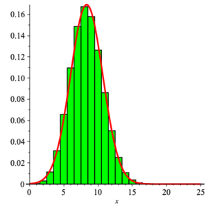
Here is the graph of the density function for the discrete random variable $\displaystyle{ {\rm binom}(25,\textstyle{\frac{1}{3}}) }$ compared with that for the continuous random variable $\displaystyle{ Z_{\frac{25}{3} , \frac{5}{3}\,\sqrt{2}} }\; $ .

As an example, consider the following problem.
Example: The incidence of color blindness in a population is $10\%\;$ . From a survey of $50,000$ members of this population, approximate the probability that the number of color blind survey participants is less than $4,900\;$ . Approximate the probability that the number of color blind participants is greater than $5,200\;$ .
Whether or not one person from the survey is color blind is a random variable with Bernoulli density function ${\rm Bernoulli}(x;.1)\,$ , where $1$ indicates color blind and $0$ indicates not. Thus the number of people color blind from a sample of size $50,000$ is a random variable with density ${\rm binom}(k;50000,.1)$ given by
$$
{\rm binom}(k;50000,.1) =\left( \begin{array}{c} 50000 \\ k \end{array} \right)\, (.9)^{50000-k}\, (.1)^k \,\text{,}
$$
hardly inviting. The probability that less than $4,900$ survey participants are color blind is
$$
\sum_{k=0}^{4899}\, \left( \begin{array}{c} 50000 \\ k \end{array} \right)\, (.9)^{50000-k}\, (.1)^k \,\text{,}
$$
again, not a convenient number to obtain.
Instead, since we know the mean and standard deviation of ${\rm binom}(k;50000,.1)\,$ , i.e.
$$
\mu = 50000\cdot 0.1 =5000 \qquad \text{and} \qquad
\sigma =\sqrt{50000\cdot 0.1\cdot (1-0.1)} \doteq 67.1 \,\text{,}
$$
we approximate
$$
\sum_{k=0}^{4899}\, \left( \begin{array}{c} 50000 \\ k \end{array} \right)\, (.9)^{50000-k}\, (.1)^k \approx P\left( 67.1\, Z_{0,1} +5000 \lt 4899.5\right) =P\left( 67.1\, Z_{0,1} \lt -100.5\right) = P\left( Z_{0,1} \lt -1.4978\right) \;\text{.}
$$
We calculate this to be
$$ P\left( Z_{0,1} \lt -1.4978\right) \doteq 0.0671 \;\text{.} $$
That is, we have determined that there is less than a seven percent chance that the number of color blind people in the population will be less than $4,900\;$ . This should be compared to the actual value
$$
\sum_{k=0}^{4899}\, \left( \begin{array}{c} 50000 \\ k \end{array} \right)\, (.9)^{50000-k}\, (.1)^k \doteq 0.0667 \;\text{.}
$$
This took a computer algebra system over an hour to obtain.
Similarly, the probability that the number of color blind participants is greater than $5,200$ is approximated by
$$
\sum_{k=5201}^{50000}\, \left( \begin{array}{c} 50000 \\ k \end{array} \right)\, (.9)^{50000-k}\, (.1)^k \approx P\left( 67.1\, Z_{0,1} +5000 \gt 5200.5\right) = P\left( Z_{0,1} \gt 2.9881\right) \doteq 0.0014 \;\text{.}
$$
Again, the computation of the actual value is prohibitive. Using much time with a computer algebra system we obtain the actual value
$$
\sum_{k=5201}^{50000}\, \left( \begin{array}{c} 50000 \\ k \end{array} \right)\, (.9)^{50000-k}\, (.1)^k \doteq 0.0015 \;\text{.}
$$
Here is an example illustrating how we can use normal approximation to assess whether or not a game is fair.
Problem: A fair coin is flipped $1000$ times, Approximate the probability that heads occurs at most $n$ times. What value of $n$ gives the approximation $95\%\;$ ? $99\%\;$ ? If a coin is flipped $1000$ times and comes up heads $532$ times, is it reasonable to think that it is a fair coin?
On flipping a fair coin $1000$ times, the probability of getting heads $k$ times is
$$
{\rm binom}(k;1000,0.5) =\left( \begin{array}{c} 1000 \\ k \end{array} \right)\, (.5)^{1000} \;\text{.}
$$
It follows that the probability of getting heads at most $k$ times is
$$ \sum_{k=0}^n\, \left( \begin{array}{c} 1000 \\ k \end{array} \right)\, (.5)^{1000} \;\text{.} $$
This can be very unpleasant to calculate explicitly. Knowing that ${\rm binom}(1000,.5)$ has mean $\mu =1000\cdot (.5) =500$ and standard deviation $\displaystyle{ \sqrt{1000\cdot ( .5)^2 } =5\,\sqrt{10} }\,$ , we instead use the approximation
$$ Z_{500,5\,\sqrt{10}} = 5\,\sqrt{10}\cdot Z_{0,1} +500 \,\text{,} $$
and determine that the desired probability is approximately
$$
P\left( Z_{500,5\,\sqrt{10}} \lt n+\textstyle{\frac{1}{2}} \right)
= P\left( Z_{0,1} \lt \frac{\left(n+\frac{1}{2}\right) -500}{5\,\sqrt{10}} \right)
=\int_{-\infty}^{\frac{\left(n+\frac{1}{2}\right) -500}{5\,\sqrt{10}}}\, \frac{1}{\sqrt{2\,\pi}}\, {\rm e}^{-\frac{x^2}{2}}\, {\rm d}x \;\text{.}
$$
We can obtain the probability using, for example, the cumulative standard normal distribution function NORMSDIST(x) in spreadsheet applications. Thus, if $n=520\,$ , then the probability that ${\rm binom}(1000,0.5)$ assumes a value no greater than $520$ is approximately
$$
\int_{-\infty}^{\frac{\left(520+\frac{1}{2}\right) -500}{5\,\sqrt{10}}}\, \frac{1}{\sqrt{2\,\pi}}\, {\rm e}^{-\frac{x^2}{2}}\, {\rm d}x =\int_{-\infty}^{1.9265}\, \frac{1}{\sqrt{2\,\pi}}\, {\rm e}^{-\frac{x^2}{2}}\, {\rm d}x =\text{NORMSDIST(1.9265)} =0.9026 \;\text{.}
$$
The $x$ value for which
$$ \int_{-\infty}^{x}\, {\rm e}^{-\frac{x^2}{2}}\, {\rm d}x =0.95 $$
is approximately $x =1.6449\,$ , so
$$
\int_{-\infty}^{\frac{\left( n+\frac{1}{2}\right) -500}{5\,\sqrt{10}}}\, \frac{1}{\sqrt{2\,\pi}}\, {\rm e}^{-\frac{x^2}{2}}\, {\rm d}x =0.95
$$
when
$$ \frac{\left( n+\frac{1}{2}\right) -500}{5\,\sqrt{10}} =1.6449 \;\text{.}$$
we solve this for $n$ to find that
$$ n =525.508 \;\text{.} $$
So, that the number of heads occurring is greater than $525$ happens less than $5\%$ of the time.
The $x$ value for which
$$ \int_{-\infty}^{x}\, {\rm e}^{-\frac{x^2}{2}}\, {\rm d}x =0.99 $$
is approximately $x =2.3263\,$ , so
$$
\int_{-\infty}^{\frac{\left( n+\frac{1}{2}\right) -500}{5\,\sqrt{10}}}\, \frac{1}{\sqrt{2\,\pi}}\, {\rm e}^{-\frac{x^2}{2}}\, {\rm d}x =0.99
$$
when
$$ \frac{\left( n+\frac{1}{2}\right) -500}{5\,\sqrt{10}} =2.3263 \;\text{.}$$
we solve this for $n$ to find that
$$ n =536.282 \;\text{.} $$
So, that the number of heads occurring is greater than $536$ happens less than $1\%$ of the time.
When on a thousand flips a coin comes up $532$ times, and we ask if it is reasonable to assume that the coin is fair, we need to agree on what makes for “reasonable”. If we agree that the number of heads be within a $1$-out-of-$20$ range, then $532 \gt 525$ and this is too many heads to be acceptable. If we agree that the number of heads be within a $1$-out-of-$100$ range, then $532 \lt 536$ and this is few enough heads to be accepted.
Here is a spreadsheet which runs the following experiment: pick one of $0$ or $1$ with equal probability a thousand times (think of this as a coin flip where $1$ means heads). This is done in cells D3:D1002. Then count the number of times $1$ occurs. This is given in cell D1. Perform this experiment five hundred times (columns D through SI). The number of times that the experiment results in greater than $525$ heads is given in cell B1. Compare this number with $25$ – that is, $\, 5\%$ of the experiments. The number of times that the experiment results in greater than $536$ heads is given in cell B2. Compare this number with $5$ $#8211; that is, $\, 1\%$ of the experiments.
Click here to open a copy of this so you can experiment with it. You will need to be signed in to a Google account.

