Often times we will want to perform computations to identify features of a probability distribution.   As an abstract example, given a process or experiment where various outcomes are numbers occurring according to a probability distribution, we may wish to compute the squares of those numbers.   Or, as a more concrete example, we may have different payouts according to various outcomes of a Las Vegas table game and want to consider all of those possible payouts at once for the purposes of determining a betting strategy.   Since we don’t know up front what the result of the experiment is going to be, we want to perform these computations while leaving the outcome variable.   The language for such is that of random variables.

Definition: A random variable is a real valued function defined on a sample space.   Since a sample space is the collection of possible outcomes for an experiment, another way to think of this is as a function whose result is determined by the outcome of the experiment.

That is, for each possible outcome of our process/experiment we have a value.   For example, consider the sample space of results on rolling two dice.   There are thirty-six possible outcomes for this experiment.   The sum of the values on the two dice is a function associating a number with each of the possible outcomes, and these numbers are integers from   $2$   to   $12$ .   As another example, consider a lottery where twenty tickets are sold for   $\mathrm{\$}2$   per ticket.   On drawing, the holder of the winning ticket gets   $\mathrm{\$}25$   (and so has gained   $\mathrm{\$}23$ ), and everyone else gets nothing and is thus out   $\mathrm{\$}2$ .   Thus there are twenty different outcomes, but if I buy a ticket the payout function is   $-\mathrm{\$}2$   for nineteen of the possible outcomes, and   $\mathrm{\$}23$   for the rare case that the winning ticket is mine.

The two examples above are examples of discrete random variables, as they have a finite (or countably infinite   –   as will be discussed in a moment) number of possible values.   We take this as the definition of a discrete random variable.   For an example of a discrete random variable which can take on any of infinite number of possible values, consider the game where one flips a coin repeatedly until it lands heads-up.   Count the number of flips it takes for this to happen.   The value of this random variable is one of the infinitely many values   $1$ , $2$ , $3$ , … .

There are other random variables which can take on values throughout an interval.   These are called continuous random variables.   As an example, suppose a dart is thrown at a dartboard of radius ten inches.   The function which assigns to the throw the distance of the dart from the center of the board is a random variable which can take any value between   $0$   and   $10$ .   Or suppose we ask where on a five kilometer stretch of highway the next automobile accident will occur.   This is a random variable which assigns to the accident a number between   $0$   and   $5$   when we measure in kilometers, or between   $0$   and   $5000$   if we measure in meters.

Functions of a Random Variable   Since we can post-compose any function   $X:S\to \mathbb{R}$   with a real-valued function   $g:\mathbb{R}\to \mathbb{R}$ , we can discuss the new random variable   $g(X)$   as a function of our original random variable   $X$ .

For example, consider the following lottery game: we pay two dollars to roll a die.   If the die comes up   $6$   we get back   $\mathrm{\$}6$   (so we’ve made   $\mathrm{\$}5$ ).   If the die comes up   $5$   we get back   $\mathrm{\$}4$   (so we’ve made   $\mathrm{\$}3$ ).   If it comes up any other number we lose our original payment.   The payout is described by the function   $X$   which assigns the value   $-1$   to the possible outcomes   $1$ , … , $4$ , the value   $3$   to the outcome   $5$ , and the value   $5$   to the outcome   $6$ .   That is, $X$   takes on value   $-1$   with probability   $\frac{4}{6}=\frac{2}{3}$ , value   $3$   with probability   $\frac{1}{6}$ , and value   $5$   with probability   $\frac{1}{6}$ .   Now suppose that there is a tax on winnings, which demands twenty percent of anything over three dollars, and ten percent of any winnings no greater than three dollars.   This effects us, only if we roll a   $5$   or a   $6$ .   Call this new function the taxation function:
$$t(X)=\{\begin{array}{ccc}0& & X\le 0\\ .1X& & 0<X\le 3\\ .2X& & X>3\end{array}\text{.}$$
With this, we see that we will pay no taxes with probability   $\frac{2}{3}$   (i.e. when we roll   $1$ , … , $4$ ), pay a tax of   $0.30$   with probability   $\frac{1}{6}$   (when we roll   $5$ ), and pay a tax of   $1.00$   with probability   $\frac{1}{6}$   (when we roll   $6$ ).   We could also consider the gain function   $g(X)$   –   the function telling us what our take-home is out of the game.   The reader can check that this function is
$$g(X)=\{\begin{array}{ccc}-1& & X\le 0\\ .9X& & 0<X\le 3\\ .8X& & X>3\end{array}\text{.}$$

Sometimes two different processes can give rise to random variables assuming the same points in   $\mathbb{R}$   with the same probabilities.   A simple example is the following: consider the two experiments of flipping a coin and drawing from a deck of cards.   In the first, let   $X$ be the random variable which assigns value   $0$   if the flip comes up tails and   $1$   if the flip comes up heads. In the second, let   $Y$   be the random variable which assigns   $0$   if the drawn card is red and   $1$   if it is black.   In both cases, the values assumed by the random variable are   $0$   and   $1$ , each with probability   $\frac{1}{2}$ . We will consider these random variables to be equivalent, as if we are presented with a string of   $0$s and   $1$s as outcomes for our experiment, we cannot distinguish flips from card draws. We will thus think of random variables as subsets of the real numbers with probabilities assigned to the elements of the subset.   We can then attach such a subset/probability pair to experiments as necessary.   For example, the subset   $\{1,2,3,4,5,6\}$   of   $\mathbb{R}$ , with probability   $\frac{1}{6}$   attached to each of these values, can be used to describe the roll of a die.   Henceforth, it is such subsets of   $\mathbb{R}$ , with non-negative values (probabilities) assigned to them, satisfying the axioms of probability that we will mean when discussing random variables.

If we have a continuous random variable, the definition of a random variable must be slightly different.   In this case, no value is assigned to individual points of our subset of   $\mathbb{R}$ .   Rather, we will say what probability there is for   $X$   to take values in various intervals.   Thus we can have a random variable which takes values in the interval   $[10,15]$ , and the probability that it takes a value in   $[a,b]$   (assuming that   $10\le a\le b\le 15$ ) will be given as   $P(a\le X\le b)=\frac{b-a}{5}$ .

For these to make sense, we need to ensure that the rules of probability are respected.   Thus we need to make sure that for no point (discrete case) or interval (continuous case) is the probability ever negative, and that the total probability is   $1$ .

Test for Random Variable   There is a simple way to determine if a function   $X$   is a properly defined random variable.

• If   $X$   (discrete) takes values   ${\displaystyle x_1}$ , ${\displaystyle x_2}$ , … with probabilities   ${\displaystyle P(X=x_1)=p_1}$ ,
  ${\displaystyle P(X=x_2)=p_2}$ , … , we need
  1. for each   $i$ , ${\displaystyle p_i\ge 0}$ , and
  2. that   ${\displaystyle \sum _i{p}_i=1}$ .
• If   $X$   (continuous), then we need
  1. for each interval   $[a,b]$   that   $P(a\le X\le b)\ge 0$ , and
  2. that   $P(-\mathrm{\infty }<X<\mathrm{\infty })=1$ .

In the above example, we saw that it was important to understand what values can be assumed by a random variable, and with what probabilities those values can be assumed.   The following discussion is about precisely this: how we keep track of the possible values of a random variable and the probabilities with which those values can be attained.

Density and Distribution

Given a random variable, we wish to keep track of what values it can assume and with what probability.   Two tools are commonly used here: density and distribution.   We will discuss these one at a time, and describe the relationship between the two.

Given a finite sample space, each of the possible outcomes has a specific probability.   Thus, denoting our random variable by   $X$   (so that   $X:S\to \mathbb{R}$ ), we know that   $X$   takes on a finite number of possible values.   Each of these has a probability of occurring.   This set of values, along with their probabilities, is called the density of   $X$ .   For example, consider the function which totals the values on rolling two standard six-sided dice.   There are thirty-six possible outcomes for the roll of two dice, as indicated below.
$$\begin{array}{ccccccc}{}_{\mathrm{\#}2}{\backslash }^{\mathrm{\#}1}& 1& 2& 3& 4& 5& 6\\ 1& (1,1)& (2,1)& (3,1)& (4,1)& (5,1)& (6,1)\\ 2& (1,2)& (2,2)& (3,2)& (4,2)& (5,2)& (6,2)\\ 3& (1,3)& (2,3)& (3,3)& (4,3)& (5,3)& (6,3)\\ 4& (1,4)& (2,4)& (3,4)& (4,4)& (5,4)& (6,4)\\ 5& (1,5)& (2,5)& (3,5)& (4,5)& (5,5)& (6,5)\\ 6& (1,6)& (2,6)& (3,6)& (4,6)& (5,6)& (6,6)\end{array}$$
But there are only eleven possible outcomes for the sum of their two values.   The possible sums are   $1$ , $2$ , $3$ , $4$ , $5$ , and   $6$ .   The pairs whose values sum to   $6$   are highlighted in blue below, and those summing to   $7$   are highlighted in red.
$$\begin{array}{ccccccc}{}_{\mathrm{\#}2}{\backslash }^{\mathrm{\#}1}& 1& 2& 3& 4& 5& 6\\ 1& (1,1)& (2,1)& (3,1)& (4,1)& (5,1)& (6,1)\\ 2& (1,2)& (2,2)& (3,2)& (4,2)& (5,2)& (6,2)\\ 3& (1,3)& (2,3)& (3,3)& (4,3)& (5,3)& (6,3)\\ 4& (1,4)& (2,4)& (3,4)& (4,4)& (5,4)& (6,4)\\ 5& (1,5)& (2,5)& (3,5)& (4,5)& (5,5)& (6,5)\\ 6& (1,6)& (2,6)& (3,6)& (4,6)& (5,6)& (6,6)\end{array}$$

We see that five out of the thirty-six equally likely rolls yield a sum of   $6$ , and six yield the sum   $7$ .   Thus the probability that the sum is   $6$   is   $\frac{5}{36}$ , and that the sum is   $7$   is   $\frac{6}{36}=\frac{1}{6}$ .   In fact, here are the eleven possible sums with their probabilities of occurring.
$$\begin{array}{cccccccccccc}\mathbf{\text{sum}}& 2& 3& 4& 5& 6& 7& 8& 9& 10& 11& 12\\ \mathbf{\text{probability}}& \frac{1}{36}& \frac{2}{36}=\frac{1}{18}& \frac{3}{36}=\frac{1}{12}& \frac{4}{36}=\frac{1}{9}& \frac{5}{36}& \frac{6}{36}=\frac{1}{6}& \frac{5}{36}& \frac{4}{36}=\frac{1}{9}& \frac{3}{36}=\frac{1}{12}& \frac{2}{36}=\frac{1}{18}& \frac{1}{36}\end{array}$$

For a discrete random variable   $X$ , such a compilation of values and probabilities is called the density of   $X$ .   It will usually be given with increasing values.   We note, consistent with our test for random variables above, that the sum of probabilities is   $1$ .   Here this is seen as
$$\frac{1}{36}+\frac{2}{36}+\frac{3}{36}+\frac{4}{36}+\frac{5}{36}+\frac{6}{36}+\frac{5}{36}+\frac{4}{36}+\frac{3}{36}+\frac{2}{36}+\frac{1}{36}=\frac{36}{36}=1\text{.}$$

The term “density” apparently comes from the way one records such information for continuous random variables.   Given a continuous random variable   $X$ , we cannot assign assign a probability to   $X$   assuming a specific value point in this case (based on the subtle notion of non-countable sets   –   not a discussion for this forum).   Instead we describe the “thickness” of probability near to a point by giving a non-negative function   $p(x)$   so that   $X$   takes on a value in interval   $[a,b]$   with probability
$$P(X\in [a,b])={\int }_a^{b}p(x)\mathrm{d}x\text{.}$$
That   $p(x)\ge 0$   implies that   $P(X\in [a,b])\ge 0$ .   Our compatibility condition becomes
$${\int }_{-\mathrm{\infty }}^{\mathrm{\infty }}p(x)\mathrm{d}x=1\text{.}$$
With this in mind, one might consider discrete probability densities as a sort of coagulation of continuous probability at specific values.

Examples: Compatibility Condition for Discrete and Continuous Probability Densities

Consider the following two problems.

Discrete Problem   Suppose that we have a process that takes as many steps as necessary to finish   –   i.e. the process could finish after one step, or after two, or after three, etc.   Suppose we further know that the process must eventually finish, and that the probability of finishing after   $n+1$   steps is half of that of finishing after   $n$   steps.   What is the probability of finishing at any particular point of the process?

One way to approach this is to observe that we do not know the probability that the process ends after the first step.   Letting   $X$   be the random variable describing the number of steps needed for our process to finish, we denote   $P(X=1)$   by   $c$ , this unknown value.   Once we know this, we get   $P(X=2)=\frac{1}{2}\cdot c$ , $P(X=3)={\left(\frac{1}{2}\right)}^2\cdot c$ , etc., and we can compute the probability that the process stops after any particular step.   Our issue is thus to compute   $c$ .

We compute   $c$   by remembering that we have a compatibility condition:
$$\sum _{k=1}^{\mathrm{\infty }}P(X=k)=1\text{,}$$
which we can identify as
$$c+\frac{1}{2}\cdot c+{\left(\frac{1}{2}\right)}^2\cdot c+\cdots =c\cdot \sum _{k=0}^{\mathrm{\infty }}{\left(\frac{1}{2}\right)}^k=1\text{.}$$
But this sum is a geometric series, whose sum is well understood.   In fact, here
$$\sum _{k=0}^{\mathrm{\infty }}{\left(\frac{1}{2}\right)}^k=\frac{1}{1-\frac{1}{2}}=2\text{,}$$
so that our compatibility condition becomes
$$c\cdot 2=1\text{,}$$
and we see that   $c=\frac{1}{2}$ .   Thus the probability of the process stopping after   $k$   steps is
$$P(X=k)={\left(\frac{1}{2}\right)}^{k-1}\cdot c={\left(\frac{1}{2}\right)}^{k-1}\cdot \frac{1}{2}={\left(\frac{1}{2}\right)}^k\text{.}$$

Continuous Problem   Suppose that we have an experiment that gives outcomes between   $0$   and   $1$ .   Data collection shows that the experiment yields outcomes concentrated near to   $\frac{1}{2}$   and tapering off at   $0$   and   $1$ .   The function   $x(1-x)$   has this property (graph shown below), so we wish to use   $cx(1-x)$   as probability density function modeling the outcomes of our experiment.   What value of   $c$   must we take?

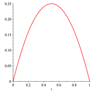
plot of   $x(1-x)$   for   $x\in [0,1]$

The compatibility condition tells us that we need
$${\int }_{-\mathrm{\infty }}^{\mathrm{\infty }}cx(1-x)\mathrm{d}x={\int }_0^{1}cx(1-x)\mathrm{d}x=1\text{.}$$
But
$${\int }_0^{1}x(1-x)\mathrm{d}x=\frac{1}{6}\text{,}$$
so we need   $c=6$   to satisfy the compatibility condition.   Thus we take   $f(x)=6x(1-x)$   as the desired model for density of the outcomes of our experiment.

There is another notion of how probability is apportioned to the values of a random variable.   This is called the probability distribution.

Probability Distribution

The distribution of a random variable   $X$   is defined as follows.

• If   $X$   is discrete, taking values   $x_1$ , $x_2$ , … , with probabilities   $p_1$ , $p_2$ , … , then the distribution function is
  $$\mathrm{D}\mathrm{F}(x;X)=P(X\le x)=\sum _{x_i\le x}{p}_i\text{,}$$
• and if   $X$   is continuous with density function   $p(x)$ , then its distribution function is
  $$\mathrm{D}\mathrm{F}(x;X)=P(X\le x)={\int }_{-\mathrm{\infty }}^{x}p(x)\mathrm{d}x\text{.}$$

That is, the distribution function   $\mathrm{D}\mathrm{F}(x;X)$   records the probability that   $X$   takes on values no greater than   $x$ .   The compatibility condition implies that
$$\underset{x\to +\mathrm{\infty }}{lim}\mathrm{D}\mathrm{F}(x;X)=1\text{,}$$
as the probability is   $1$   that   $X$   takes on some value.   As with density functions, we will suppress the mention of random variable   $X$   if it is understood.

By way of examples, we construct the distribution functions   $\mathrm{D}\mathrm{F}(x;X)$   for the two examples considered above when examining the compatibility condition.

• Discrete Example:   We had the density function  
  $$p(x)=\{\begin{array}{cc}\frac{1}{2^x}& x\in {\mathbb{Z}}_{+}\\ & \\ 0& \text{otherwise}\end{array}\text{.}$$
  Thus the distribution function is
  $$\mathrm{D}\mathrm{F}(x)=\{\begin{array}{cc}0& x<1\\ & \\ \frac{2^k-1}{2^k}& x\in [k,k+1)\end{array}\text{,}$$
  with the following graph.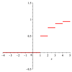
  

  graph of distribution function

• Continuous Example:   We had the density function  
  $$p(x)=\{\begin{array}{cc}6x(1-x)& x\in [0,1]\\ & \\ 0& \text{otherwise}\end{array}\text{.}$$
  Thus the distribution function is
  $$\mathrm{D}\mathrm{F}(x)=\{\begin{array}{cc}0& x\le 0\\ & \\ x^2(3-2x)& x\in (0,1)\\ & \\ 1& x\ge 1\end{array}\text{,}$$
  with the following graph.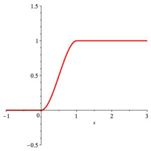
  

  graph of distribution function

We note that the density function   $p(x)$   can be obtained from the distribution function   $\mathrm{D}\mathrm{F}(x)$   by a straightforward procedure.

• If   $X$   is discrete then   $p\left(x_0\right)=\mathrm{D}\mathrm{F}\left(x_0\right)-{\displaystyle \underset{x<img\; draggable="false"\; role="img"\; class="emoji"\; alt="\nearrow "\; src="https://s.w.org/images/core/emoji/15.0.3/svg/2197.svg">x_0}{lim}\mathrm{D}\mathrm{F}(x)}$ .
• If   $X$   is continuous then   $p\left(x_0\right)={\displaystyle {\frac{\mathrm{d}\phantom{x}}{\mathrm{d}x}\mathrm{D}\mathrm{F}(x)|}_{x=x_0}}$ .

The language here is sometimes a bit confusing, as different groups of people came at these ideas
from different points of view.   Sometimes our notion of probability density is called “probabilty distribution”, and our notion of probability distribution is then called “cumulative probability distribution”.   Neither is right or wrong.   The choice of terminology is a convention, and in any setting the attentive participant must clarify what the words being used mean.   We will use the language presented here, because it is more common in mathematics and natural sciences.