There are several continuous random variables which occur routinely, generally used in situations where there is a continuum of possible outcomes   –   a collection of possible outcomes requiring at least an interval of   $\mathbb{R}$   to parameterize.   Anyone wishing to (or needing to) use mathematical statistics should be familiar with at least the following distributions.

Rectangular (or Uniform) Random Variables

Situations where a measured quantity is known to be in a certain interval   $[a,b]\,$ , with all values of the interval equally likely, are modelled by rectangular random variables.   Let   $X$   be a random variable with density $$ {\rm U}_{[a,b]}(x) =\left\{ \begin{array}{cc} \frac{1}{b-a} & a\le x\le b \\ & \\ 0 & \text{elsewhere} \end{array} \right. $$ (We use   $U$   for “uniform”.)

Example:   Position of a Vehicle

The position of a car at a given moment along a stretch of road marked with mile markers from   $0$   to   $20$   can be modeled by a random variable with uniform density   $\displaystyle{ {\rm U}_{[0,20]} }\;$ .

The main descriptors of a uniform random variable are determined below.

Mean of a Uniform Random Variable

The mean of the uniform random density   $\displaystyle{ {\rm U}_{[a,b]} }$   is computed by $$ \begin{array}{rl} \mu & =\frac{1}{b-a}\, \int_a^b x\, {\rm d}x \\ & \\ & =\frac{1}{b-a}\cdot\frac{b^2 -a^2}{2} \\ & \\ & =\frac{a+b}{2} \; \text{.} \end{array} $$ That is, the average value of such a rectangular density is the midpoint of the interval of possible values.

Variance of a Uniform Random Variable

The variance of the uniform random density   $\displaystyle{ {\rm U}_{[a,b]} }$   will be computed by the   $\displaystyle{ \sigma^2 =\mu_2 -\mu^2 }$   trick.   To this end, we have $$ \begin{array}{rl} \mu_2 & =\frac{1}{b-a}\, \int_a^b x^2\, {\rm d}x \\ & \\ & =\frac{1}{b-a}\cdot\frac{b^3-a^3}{3} \\ & \\ & =\frac{a^2 +a\, b +b^2}{3} \end{array} $$ So that $$ \sigma^2 =\frac{a^2 +a\, b +b^2}{3} -\left( \frac{a+b}{2} \right)^2 =\frac{(b-a)^2}{12} \;\text{.} $$ The standard deviation is then $$ \sigma =\frac{b-a}{\sqrt{12}} \;\text{.} $$

The moment generating function of a uniform random variable can be explicitly computed, and used to obtain the above values.

The Moment Generating Function of a Uniform Random Variable

Let   $X$   have density   $\displaystyle{ {\rm U}_{[a, b]} }\,$ , and   $t\neq 0\;$ .   We have the following. $$ \begin{array}{rl} M_X(t) & =E\left[ {\rm e}^{t\, X} \right] \\ & \\ & =\int_a^b\, {\rm e}^{t\, x}\,\frac{1}{b-a}\, {\rm d}x \\ & \\ & =\frac{1}{b-a}\,\int_a^b\, {\rm e}^{t\, x}\, {\rm d}x \\ & \\ & =\frac{1}{b-a}\,\frac{1}{t}\, {\rm e}^{t\, x}\Big|_{x=a}^{x=b} \\ & \\ & =\frac{1}{t\, (b-a)}\,\left( {\rm e}^{t\, b} -{\rm e}^{t\, a} \right) \end{array} $$ Thus, for example, $$ \frac{{\rm d}\phantom{t}}{{\rm d}t}\, M_X(t) =\frac{t\, \left( b\, {\rm e}^{t\, b} -a\, {\rm e}^{t\, a} \right) – \left( {\rm e}^{t\, b} -{\rm e}^{t\, a} \right)}{t^2\, (b-a)} \;\text{.} $$ We cannot evaluate this directly at   $t=0$   to obtain   $\mu\;$ .   Instead we use l’Hôpital’s rule to obtain $$ \begin{array}{rl} \mu =\lim_{t\to 0}\, \frac{{\rm d}\phantom{t}}{{\rm d}t}\, M_X(t) & =\lim_{t\to 0}\, \frac{b^2\, {\rm e}^{b\, t} -a^2\, {\rm e}^{a\, t}}{2\, (b-a)} \\ & \\ & =\frac{b^2 -a^2}{2\, (b-a)} \\ & \\ & =\frac{b+a}{2} \;\text{.} \end{array} $$ This agrees with our previous computation.

Exponential Random Variables

Exponential random variables arise when considering how long it will take for an event to occur   –   the first person to enter a supermarket check-out line, for example.   Or the failure of a piece of equipment.   Or the radioactive decay of a particle.   Their density functions are given by $$ {\rm Exp}_\lambda(x) =\left\{ \begin{array}{cc} \lambda\, {\rm e}^{-\lambda\, x} & x\gt 0 \\ & \\ 0 & \text{otherwise} \end{array} \right. \qquad (\lambda \gt 0)\;\text{.} $$

The main descriptors of exponential random variables are determined below.

Mean of Exponential Random Variables

The mean of the exponential random density   ${\rm Exp}_\lambda$   is $$ \begin{array}{rl} \mu & =\int_0^{\infty}\, x\,\lambda\, {\rm e}^{-\lambda\, x}\, {\rm d}x \\ & \\ & =\frac{1}{\lambda} \; \text{.} \end{array} $$ That is, the average value of such an exponential random variables is precisely the reciprocal of its parameter   $\lambda\;$ .   Thus one often sees exponential random variables written as   ${\rm Exp}_{\frac{1}{\mu}}\;$ .

Variance of Exponential Random Variables

The variance of the exponential random density   $\displaystyle{ {\rm Exp}_{\frac{1}{\mu}} }$   will be computed by the   $\displaystyle{ \sigma^2 =\mu_2 -\mu^2 }$   trick.   To this end, we have $$ \begin{array}{rl} \mu_2 & =\int_0^{\infty}\, x^2\cdot \frac{1}{\mu}\, {\rm e}^{-\frac{x}{\mu}}\, {\rm d}x \\ & \\ & =2\,\mu^2 \end{array} \;\text{.} $$ Thus $$ \sigma^2 =2\,\mu^2 -(\mu)^2 =\mu^2 \;\text{.} $$ The standard deviation is then $$ \sigma =\mu =\frac{1}{\lambda} \;\text{.} $$

Example:   The average waiting time for calls at a help line is five minutes.   What is the probability that a call will arrive in the next three minutes?   What is the probability that no calls will arrive in the next eight minutes?

With   $\mu =5\,$ , we have $$ P( 0\le X\lt 3) =\int_0^3\, \frac{1}{5}\,\exp\left( -\frac{x}{5} \right)\, {\rm d}x =1-\exp\left( -\frac{3}{5} \right) \doteq 0.4512 $$ and $$ P( X\gt 8) =\int_8^{\infty}\, \frac{1}{5}\,\exp\left( -\frac{x}{5} \right)\, {\rm d}x =\exp\left( -\frac{8}{5} \right) \doteq 0.2019 \;\text{.} $$ Note that this last computation can be obtained by $$ P( X\gt 8) =1-P( X\le 8) = 1- \int_0^8\, \frac{1}{5}\,\exp\left( -\frac{x}{5} \right)\, {\rm d}x \doteq 1- 0.7981 =0.2019 \;\text{.} $$

Computing Probabilities for Exponential Random Variables with Spreadsheets

Computations of density and distribution functions for exponential random variables are easily performed within spreadsheets.   The important thing to remember is that EXP means the exponential function, so a new term must be used.   This is EXPONDIST.   Thus we have “=EXPONDIST($x$, $\lambda$, 0)” yields the density function   $\displaystyle{ {\rm Exp}_{\lambda}(x) =\lambda\,\exp(-\lambda\, x) }\,$ , while “=EXPONDIST($x$, $\lambda$, 1)” gives the distribution function   $\displaystyle{ \int_0^x\, \lambda\,\exp(-\lambda\, t)\, {\rm d}t =1-\exp(-\lambda\, x) }\;$ .

This can be seen in the following spreadsheet.   A value of   $\lambda$   ( $\,\in [\frac{1}{2}, 2]\,$ ) is given in cell B1, and a value of   $x$   ( $\,\in [1, 5]\,$ ) is given in cell B2.   If   $X$   represents an exponential random variable with   $\lambda$   the value in B1, we display several computations.   In cell E1 you will find the value of the density function given by “=EXPONDIST(B2, B1, 0)”, and in cell E2 you will find a check of this with “=B1*EXP(-B1*B2)”.   Notice that the cells E1 and E2 have been identically colored so as to be easily compared.   In E3 you will find the probability   $P( X\lt B2)$   given by “=EXPONDIST(B2, B1, 1)”, in cell E4 you will find the probability   $P( X\ge B2)$   given by “=1-EXPONDIST(B2, B1, 1)”, and in E5 a check that this last can be obtained by “=EXP(-B2*B1)”.   Cells E4 and E5 have been identically colored so as to be easily compared.

Click here to open a copy of this so you can experiment with it. You will need to be signed in to a Google account.

Normal Random Variables

Normal random variables are an important class of continuous random variables whose value will become apparent shortly.   Consider the continuous random variable   $\displaystyle{ Z_{a,b} }$   (for   $a\in\mathbb{R}\,$ , $\,\displaystyle{ b\in\mathbb{R}_+ }\,$ ) whose density function is given by $$ {\rm norm}_{a,b}(x) =\frac{1}{b\, \sqrt{2\,\pi}}\, \exp\left(-\frac{1}{2}\,\left(\frac{x- a}{b}\right)^2\right) \, \text{,} $$ with cumulative distribution $$ \frac{1}{b \,\sqrt{2\,\pi}}\, \int_{-\infty}^x\, \exp\left(-\frac{1}{2}\,\left(\frac{t- a}{b}\right)^2\right) \, {\rm d}t \; \text{.} $$

The distribution   $\displaystyle{ Z_{0,1} }\,$ , with density $$ Z_{0,1}(x) =\frac{1}{\sqrt{2\,\pi}}\, \exp\left(-\frac{x^2}{2}\right) $$ is commonly called standard normal.   Normal random variables may have subscripts suppressed (i.e. denoted by   $Z\,$ ) if   $a$   and   $b$   are understood.

For these to truly be random variables, we need that the associated densities are non-negative and have integrals $$ \frac{1}{b \,\sqrt{2\,\pi}}\, \int_{-\infty}^{\infty}\, \exp\left( -\frac{1}{2}\,\left(\frac{t- a}{b}\right)^2 \right) \, {\rm d}t =1 \;\text{.} $$ That the densities are actually positive follows from the fact that exponential functions are always positive, and that the integral   $=1$   follows from the following rather advanced fact. Fact:   $\displaystyle{ \int_{-\infty}^{\infty}\, \exp\left(-x^2\right)\, {\rm d}x =\sqrt{\pi} }\,$ , found, for example, at https://en.wikipedia.org/wiki/Gaussian_integral.

A derivation, and several consequences, of the fact that   $\displaystyle{ \int_{-\infty}^{\infty}\, \exp\left(-x^2\right)\, {\rm d}x =\sqrt{\pi} }\;$

First we show why the integral has the value claimed.

To this end, let   $\displaystyle{ V =\int_{-\infty}^{\infty}\, \exp\left(-x^2\right)\, {\rm d}x }\;$ .   Then $$ \begin{array}{rl} V^2 & =\int_{-\infty}^{\infty}\, \exp\left(-x^2\right)\, {\rm d}x \cdot \int_{-\infty}^{\infty}\, \exp\left(-y^2\right)\, {\rm d}y \\ & \\ & =\int\int_{\mathbb{R}^2}\, \exp\left(-\left(x^2 +y^2\right)\right)\, {\rm d}A \\ & \\ & =\int_0^{2\,\pi} \left( \int_0^{\infty}\, r\,\exp\left(-r^2\right)\, {\rm d}r \right) \, {\rm d}\theta \\ & \\ & =2\,\pi\, \left( \frac{1}{2} \int_0^{\infty}\, \exp(-u)\, {\rm d}u \right) \\ & \\ & =\pi \;\text{.} \end{array} $$ So in fact   $\displaystyle{ V =\sqrt{\pi} }\,$ , and we have established the basic integral equality.

Now, let $$ t=\frac{x}{\sqrt{2}} $$ in the integral equality $$ \int_{-\infty}^{\infty}\, \exp\left(-t^2\right)\, {\rm d}t =\sqrt{\pi} \;\text{.} $$ We get $$ \frac{1}{\sqrt{2}}\, \int_{-\infty}^{\infty}\, \exp\left(-\frac{x^2}{2}\right)\, {\rm d}x =\sqrt{\pi} $$ or $$ \frac{1}{\sqrt{2\,\pi}}\, \int_{-\infty}^{\infty}\, \exp\left(-\frac{u^2}{2}\right)\, {\rm d}u =1 \;\text{.} $$ This shows that   $\displaystyle{ Z_{0,1} }$   is a probability density.

Finally, make a further change of variable   $\displaystyle{ u =\frac{s-a}{b} }$   in the last equality above.   The equality is re-expressed as $$ \int_{-\infty}^{\infty}\, \frac{1}{b\,\sqrt{2\,\pi}}\, \exp\left(-\frac{1}{2}\, \left( \frac{s-a}{b} \right)^2\right)\, {\rm d}s =1\;\text{.} $$ We see that every one of the   $\displaystyle{ Z_{a,b} }$   is also a probability density.

The main descriptors of a normal random variable are determined below. We will see that   $a=\mu$   and   $b=\sigma\;$ .   Because of this we will henceforth refer to   $\displaystyle{ Z_{\mu,\sigma} }$   instead of   $\displaystyle{ Z_{a,b}(x) }$   when values of the parameters are unknown.

The mean of   $\displaystyle{ Z_{a,b} }$   is   $a\;$ .

Here we first notice that the mean of a standard normal variable is   computed by $$ \int_{-\infty}^{\infty}\, t\,\frac{1}{\sqrt{2\,\pi}}\, \exp\left(-\frac{1}{2}\, t^2\right)\, {\rm d}t \;\text{.} $$ Since the integrand is an odd function of   $t\,$ , this integral evaluates to   $0\;$ .

To compute the mean of non-standard normal variable   $\displaystyle{ Z_{a,b} }\,$ ,   we integrate $$ \int_{-\infty}^{\infty}\, t\,\frac{1}{b\,\sqrt{2\,\pi}}\, \exp\left(-\frac{1}{2}\,\left( \frac{t-a}{b} \right)^2\right)\, {\rm d}t \;\text{.} $$ To evaluate this, we make the change of variable   $\displaystyle{ s =\frac{t-a}{b} }$   and see that the integral becomes $$ \int_{-\infty}^{\infty}\, (b\, s+a)\,\frac{1}{\sqrt{2\,\pi}}\, \exp\left(-\frac{1}{2}\, s^2\right)\, {\rm d}s \;\text{.} $$ Splitting this into two integrals $$ b\, \int_{-\infty}^{\infty}\, s\,\frac{1}{\sqrt{2\,\pi}}\, \exp\left(-\frac{1}{2}\, s^2\right)\, {\rm d}s $$ (which evaluates to   $0\,$ ), and $$ a\, \int_{-\infty}^{\infty}\,\frac{1}{\sqrt{2\,\pi}}\, \exp\left(-\frac{1}{2}\, s^2\right)\, {\rm d}s $$ (which evaluates to   $a\,$ ), we have $$ \int_{-\infty}^{\infty}\, (b\, s+a)\,\frac{1}{\sqrt{2\,\pi}}\, \exp\left(-\frac{1}{2}\, s^2\right)\, {\rm d}s =a \;\text{.} $$ That is, the mean of   $\displaystyle{ Z_{a,b} }$   is   $a\;$ .

The standard deviation of   $\displaystyle{ Z_{a,b} }$   is   $b\;$ .

Here we first notice that the mean of a standard normal variable is   computed by $$ \int_{-\infty}^{\infty}\, t\,\frac{1}{\sqrt{2\,\pi}}\, \exp\left(-\frac{1}{2}\, t^2\right)\, {\rm d}t \;\text{.} $$ Since the integrand is an odd function of   $t\,$ , this integral evaluates to   $0\;$ .

Example:   The moment generating function of   $\displaystyle{ Z_{\mu,\sigma} }$   is   $\displaystyle{ \exp\left( \mu\, t+ \frac{1}{2}\,\sigma^2\, t^2 \right) }\;$ .

To see this, we first determine the moment generating function of   $\displaystyle{ Z_{0,1} }\;$ .   A change of variables will allow us to then find the moment generating function of   $\displaystyle{ Z_{\mu,\sigma} }\;$ .

To this end, $$ \begin{array}{rl} M_{Z_{0,1}}(t) & =\int_{-\infty}^{\infty}\, {\rm e}^{t\, x}\, \frac{1}{\sqrt{2\,\pi}}\,{\rm e}^{-\frac{1}{2}\, x^2}\, {\rm d}x \\ & \\ & =\int_{-\infty}^{\infty}\, \frac{1}{\sqrt{2\,\pi}}\,{\rm e}^{-\frac{1}{2}\, \left( x^2 -2\, x\, t +t^2 -t^2 \right)}\, {\rm d}x \\ & \\ & ={\rm e}^{\frac{1}{2}\, t^2}\,\int_{-\infty}^{\infty}\, \frac{1}{\sqrt{2\,\pi}}\,{\rm e}^{-\frac{1}{2}\, (x-t)^2}\, {\rm d}x \\ & \\ & ={\rm e}^{\frac{1}{2}\, t^2} \;\text{.} \end{array} $$ and, with   $\displaystyle{ W =Z_{\mu,\sigma} }\,$ , $$ \begin{array}{rl} M_W(t) & =\int_{-\infty}^{\infty}\, {\rm e}^{t\, x}\, \frac{1}{\sigma\,\sqrt{2\,\pi}}\, {\rm e}^{-\frac{1}{2}\, \left( \frac{x-\mu}{\sigma} \right)^2}\, {\rm d}x \\ & \\ & =\int_{-\infty}^{\infty}\, \frac{1}{\sigma\,\sqrt{2\,\pi}}\, {\rm e}^{-\frac{1}{2}\, \left( \left( \frac{x-\mu}{\sigma} \right)^2 -2\,t\,x \right)}\, {\rm d}x \\ & \\ & =\int_{-\infty}^{\infty}\, \frac{1}{\sigma\,\sqrt{2\,\pi}}\, {\rm e}^{-\frac{1}{2}\, \left( \left( \frac{x-\mu}{\sigma} \right)^2 -2\,\sigma\,t\,\left( \frac{x-\mu}{\sigma} \right) +(\sigma\,t)^2 -2\,\mu\,t -\sigma^2\,t^2 \right)}\, {\rm d}x \\ & \\ & ={\rm e}^{\mu\,t +\frac{1}{2}\,\sigma^2\, t^2}\,\int_{-\infty}^{\infty}\, \frac{1}{\sqrt{2\,\pi}}\,{\rm e}^{-\frac{1}{2}\, \left( \left( \frac{x-\mu}{\sigma} \right) -\sigma\,t \right)^2}\, {\rm d}x \\ & \\ & ={\rm e}^{\mu\,t +\frac{1}{2}\,\sigma^2\, t^2} \;\text{.} \end{array} $$

What follows is a selection of probability computations with normal random variables.   These should be examined as they are standard and will be used later without hesitation.

Computations with Normal Densities

Computations with a Standard Normal Variable

For a standard normal variable   $\displaystyle{ Z_{0,1} }\,$ , we have $$ P\left( Z_{0,1} \lt a \right) =\int_{-\infty}^a\, \frac{1}{\sqrt{2\,\pi}}\,\exp\left(-\frac{x^2}{2}\right)\, {\rm d}x =P\left( Z_{0,1} \le a \right) $$ (as the probability that   $\displaystyle{ Z_{0,1} }$   takes on precisely any given value is zero).   Geometrically, this is the area under the curve   $\displaystyle{ y =\frac{1}{\sqrt{2\,\pi}}\, {\rm e}^{-\frac{x^2}{2}} }$   for   $x\lt a\;$ .   This is shown in the diagram below.

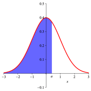
$P( Z_{0,1} \lt a) =$   shaded area

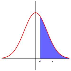
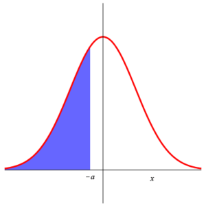
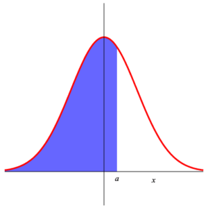
Since the function   $\displaystyle{ f\,(x) =\frac{1}{\sqrt{2\,\pi}}\, {\rm e}^{-\frac{x^2}{2}} }$   is even (i.e.   $f\,(-x) =f\,(x)\,$ ), we have $$ P\left( Z_{0,1} \gt a \right) =\int_a^{\infty}\, \frac{1}{\sqrt{2\,\pi}}\,\exp\left(-\frac{x^2}{2}\right)\, {\rm d}x =\int_{-\infty}^{-a}\, \frac{1}{\sqrt{2\,\pi}}\,\exp\left(-\frac{x^2}{2}\right)\, {\rm d}x =P\left( Z_{0,1} \le -a \right) =1- P\left( Z_{0,1} \le a \right) \;\text{.} $$ This is shown in the following illustration.

Area 1	Area 2	Area 3

Area 1   =   Area 2   =   1 – Area 3

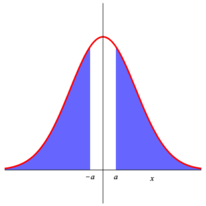
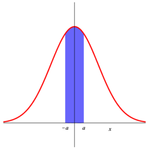
We can use these to compute   $\displaystyle{ P\left( a\lt Z_{0,1} \lt b \right) }$   for arbitrary   $a\lt b\;$ . $$ \begin{array}{rl} P\left( a\lt Z_{0,1} \lt b \right) & =\int_a^b\, \frac{1}{\sqrt{2\,\pi}}\,\exp\left(-\frac{x^2}{2}\right)\, {\rm d}x \\ & \\ & =\int_{-\infty}^b\, \frac{1}{\sqrt{2\,\pi}}\,\exp\left(-\frac{x^2}{2}\right)\, {\rm d}x -\int_{-\infty}^a\, \frac{1}{\sqrt{2\,\pi}}\,\exp\left(-\frac{x^2}{2}\right)\, {\rm d}x \\ & \\ =P\left( Z_{0,1} \le b \right) -P\left( Z_{0,1} \le a \right) \end{array} $$ Similar is the computation of   $\displaystyle{ P\left( \left| Z_{0,1} \right| \gt a \right) }$ : $$ P\left( \left| Z_{0,1} \right| \gt a \right) =1- P\left( \left| Z_{0,1} \right| \le a \right) =1- P\left( \left| Z_{0,1} \right| \le a \right) =2\, P\left( Z_{0,1}\lt -a \right) \;\text{.} $$ These can be seen in the diagram below.

Area 4	Area 5	Area 6

Area 4   =   1 – Area 5   =   2 ⋅ Area 6

The first of these computations is obtained in spreadsheets using a command such as “=NORMSDIST( )” .   The others usually require the type of arithmetic indicated above.   in the following spreadsheet we you see in cells B1 and B2 two randomly generated decimal value between   $-1$   and   $1\;$ , with the first ( $\, a\,$ ) negative and the second ( $\, b\, $ ) positive.   In cell E1 we use the command “=NORMSDIST(A1)” to generate   $\displaystyle{ P\left( Z_{0,1} \lt a \right) }$ .   In cell E2 we use the command “=NORMSDIST(-A2)” to generate   $\displaystyle{ P\left( Z_{0,1} \gt b \right) }$ .   Note that this is the same as the value in E3 obtained using “=1-NORMSDIST(A2)” .   In cell E4 we use the command “=NORMSDIST(A2)-NORMSDIST(A1)” to generate   $\displaystyle{ P\left( a \lt Z_{0,1} \lt b \right) }$ .   In cell E5 we use the command “=2*(1-NORMSDIST(A2))” to generate   $\displaystyle{ P\left( \left| Z_{0,1} \right| \gt b \right) }$ .   The spreadsheet is not performing any sort of approximation of the integral, but rather is accessing a stored table of values.  . Standard normal variables are of great enough importance that values of this awkward integral were computed using approximation methods from calculus and recorded in massive books.   Many libraries still have these books on shelves.   For our purposes, you can obtain values of the standard normal cumulative distribution function from the tool attached to this section.

Click here to open a copy of this so you can experiment with it. You will need to be signed in to a Google account.

Computations with Other Normal Variables

Computations with non-standard normal variables, similar to those for standard normal variables, are produced with linear change of variable.   Noting that with the change of variable   $\displaystyle{ s =\frac{t-\mu}{\sigma} }$   the integral $$ \int_A^B\, \frac{1}{\sigma\,\sqrt{2\,\pi}}\,\exp\left(-\frac{1}{2}\,\left(\frac{t-\mu}{\sigma}\right)^2\right)\, {\rm d}t $$ becomes $$ \int_{\frac{A-\mu}{\sigma}}^{\frac{B-\mu}{\sigma}}\, \frac{1}{\sqrt{2\,\pi}}\,\exp\left(-\frac{1}{2}\, s^2\right)\, {\rm d}s \,\text{,} $$ we interpret this as $$ P\left( A \lt Z_{\mu,\sigma}\lt B\right) =P\left( \frac{A-\mu}{\sigma} \lt Z_{0,1}\lt \frac{B-\mu}{\sigma}\right) \;\text{.} $$

Just as for standard normal variables there are spreadsheet commands to determine values of the cumulative distribution, so too do such exist for other normal variables.   Typically a command such as “=NORMDIST( )” exists in a spreadsheet.   This command returns either the density or distribution function for a prescribed normal variable, as per request.   It requires that one enter the mean and standard deviation of the normal variable, and choose the output.   In the following spreadsheet you will see in cell B1 a randomly generated number between   $-5$   and   $5\,$ , in B2 a randomly generated number between   $-2$   and   $2\,$ , and in cell B3 a randomly generated number between   $0.5$   and   $2\;$ .   In E1 you will see a number generated by the command “=NORMDIST(A1, A2, A3, 1)” which is   $\displaystyle{ P\left( Z_{A2,A3} \lt A1\right) }\;$ .   The command “=NORMDIST(A1, A2, A3, 0)” returns the density function value (so that the 0/1 in the last place indicates whether or not the density function is integrated   –   1 means yes and 0 means no).   $\displaystyle{ {\rm norm}_{A2,A3}(A1) }\;$ .   A verification of the computational trick mentioned above is shown in cell E2 where you will find a number generated by the command “=NORMSDIST((A1-A2)/A3)” .   As observed in the discussion of the command “=NORMDIST”, this is   $\displaystyle{ P\left( Z_{0,1} \lt \frac{A1-A2}{A3}\right) }\;$ .   Note that it is exactly the same as the value in E1.   (Also observe that we use subscripts “m” and “s” for   $\mu$   and   $\sigma\,$ , as Google sheets do not allow easy creation of subscripts.)

Click here to open a copy of this so you can experiment with it. You will need to be signed in to a Google account.

Two other classes of continuous random variables are included.   These will also be important in later discussions, although nowhere near as important as normal random variables.   The introductions below are brief at best, and such random variables will be discussed later as necessary.

The   $\chi^2$   class

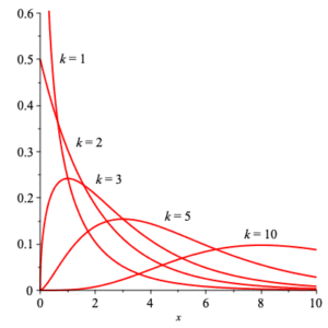
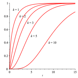
The   $\chi^2$   (read “chi-squared”) with   $k$   degrees of freedom has density function is given by $$ \chi^2(x;k) =\frac{1}{2^{k/2}\,\Gamma\left( \frac{k}{2}\right)} \, x^{\frac{k}{2} -1} \, {\rm e}^{-\frac{x}{2}} \,\text{,} $$ where   $\Gamma(x)$   is the important mathematical function $$ \Gamma(x) = \int_0^\infty\, t^{x-1}\, {\rm e}^{-t}\, {\rm d}t \;\text{.} $$ The corresponding distribution function is $$ \frac{ \gamma\left( \frac{k}{2}, \frac{x}{2} \right) }{ \Gamma\left( \frac{k}{2} \right) } \,\text{,} $$ where $$ \gamma(s,x) =\int_0^x\, t^{s-1}\, {\rm e}^{-t}\, {\rm d}t \;\text{.} $$ Plots of both density and distribution functions are shown below for   $k =1, 2, 3, 5, 10\;$ .

densities	distributions

The mean of   $\chi^2(x;k)$   can be explicitly calculated to be   $k\, $ , and the variance calculated to be   $2\, k\;$ .   The moment generating function can be explicitly determined for this family of densities: $$ MGF_{\chi^2(x;k)}(t) =(1-2\, t)^{-k/2} \;\text{.} $$

Student’s   $t$   distributions

Student’s   $t$   distribution has density function $$ T(x;\nu) =\frac{\Gamma\left( \frac{\nu +1}{2} \right)}{ \sqrt{\nu\,\pi}\,\Gamma\left( \frac{\nu}{2} \right) } \, \left( 1+\frac{x^2}{\nu}\right)^{-\frac{\nu +1}{2}} $$ and distribution function $$ \frac{1}{2} +x\,\Gamma\left( \frac{\nu +1}{2} \right)\, \frac{_2F_1\left( \frac{1}{2}, \frac{\nu +1}{2}; \frac{3}{2}; -\frac{x^2}{\nu}\right) }{ \sqrt{\nu\,\pi}\,\Gamma\left( \frac{\nu}{2} \right) } \,\text{,} $$ where   $\displaystyle{ _2F_1 }$   is a hypergeometric function.   Random variables with these density functions are often used to approximate the standard normal, and in the applet below (not currently functional) the reader can control   $\nu$   from   $1$   to   $25\;$ .   It is clear that as   $\nu$   increases the approximation to the standard normal (also plotted) improves.   In fact, the limit as   $\nu\to +\infty$   is precisely the standard normal.

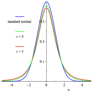
graphs of Student’s   $t$   functions for   $\nu=3$   and   $\nu=3\,$ , compared to graph of standard normal

The means of these are all   $0\,$ , and the variance is   $\frac{\nu}{\nu -2}$   as long as   $\nu \gt 2\;$ .   The moment generating function is undefined.