In an earlier section we mentioned the range of a data set. This can serve as a measure of how spread the data is. Here we introduce two refinements on the concept of spread. These are more precise measures, giving us an idea of how the data fills out the range.

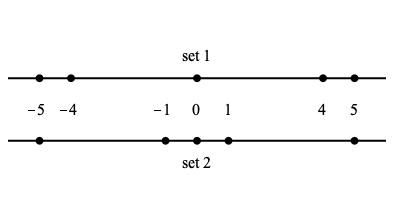
Consider the following two data sets, each containing five values. $$\begin{array}{cccccc}& x_1& x_2& x_3& x_4& x_5\\ \text{set 1}& -5& -1& 0& 1& 5\\ \text{set 2}& -5& -4& 0& 4& 5\end{array}$$ Each has   $\text{mean}=0$ , with maximum and minimum values ( $5$   and   $-5$ , respectively) in both cases being the same. That is, the range in each is exactly the same, i.e.   $5-(-5)=10$ . But there is a difference in the two data sets   –   the extent to which the data are dispersed or spread about   $0$ . Here is a graphic showing the two data sets, allowing us to visualize the dispersion in each case.

There are several measures of dispersion, but we will only concern ourselves with two closely related such measures. The variance, and its square root   –   the standard deviation. Variance is easier to calculate, but standard deviation has proper units and so is easily interpreted when visualizing data. When the standard deviation is small the data will tend to be clustered close to the mean, and when the standard deviation is large the data will tend to be more distributed away from the mean.

Variance

The variance of a set of numbers is a measure of how spread the set is about its mean. Here is an explanation of how it is computed.

Since the square of a number is a way to measure how far it is from   $0$   without concern for its sign, a reasonable measure of distance of values from the mean is the average of the square of the distance of data values from the mean of the data. In formula, this works as follows. If we have the   $n$   data values   ${\displaystyle x_1}$ , ${\displaystyle x_2}$ , … , ${\displaystyle x_n}$ , with mean $$\overline{x}=\frac{1}{n}\cdot \sum _{k=1}^n{x}_k\text{,}$$ the square of the distance of datum value   ${\displaystyle x_1}$   from   $\overline{x}$   is ${\displaystyle {(x_1-\overline{x})}^2}$ , and similarly for the other data values.   Thus the average of the   $n$   values   ${\displaystyle {(x_1-\overline{x})}^2}$ , ${\displaystyle {(x_2-\overline{x})}^2}$ , … , ${\displaystyle {(x_n-\overline{x})}^2}$   is $$\frac{{(x_1-\overline{x})}^2+{(x_2-\overline{x})}^2\cdots {(x_n-\overline{x})}^2}{n}=\frac{1}{n}\cdot \sum _{k=1}^n{(x_k-\overline{x})}^2\text{.}$$

NOTE! The above is a fine notion of dispersal of data values about the mean, except for a small issue that cannot reasonably be explained quite yet.

Because of this small issue, a variation on the above notion of dispersal is routinely used, and implemented in spreadsheets and statistical analysis packages. Given data values   ${\displaystyle x_1}$ , ${\displaystyle x_2}$ , … , ${\displaystyle x_n}$ , the variance   –   denoted by   ${\displaystyle s^2}$   (or   ${\displaystyle s_X^2}$   when we wish to acknowledge that the computation is being done using data set   $X$ )   –   will be taken as $$\mathbf{variance}=s^2=\frac{{(x_1-\overline{x})}^2+{(x_2-\overline{x})}^2\cdots {(x_n-\overline{x})}^2}{n-1}=\frac{1}{n-1}\cdot \sum _{k=1}^n{(x_k-\overline{x})}^2\text{.}$$ The only difference is that the denominator has been changed from   $n$   to   $n-1$ .

When comparing the variances of two data sets, the greater variance corresponds to data points being on average further from the mean.

Example: Find the variances of data sets 1 and 2 above and compare.

The variance of data set 1 is $$s_1^2=\frac{(-5-0{)}^2+(-1-0{)}^2+(0-0{)}^2+(1-0{)}^2+(5-0{)}^2}{5-1}=\frac{52}{4}=13\text{.}$$ The variance of data set 2 is $$s_2^2=\frac{(-5-0{)}^2+(-4-0{)}^2+(0-0{)}^2+(4-0{)}^2+(5-0{)}^2}{5-1}=\frac{82}{4}=20.5\text{.}$$ That   ${\displaystyle s_1^2<s_2^2}$   come from the fact that   ${\displaystyle x_2}$   and   ${\displaystyle x_4}$   in data set 1 are closer to the mean ( $0$ ) of set 1 than the corresponding values of set 2 are to the mean of set 2.

Spreadsheets usually allow us to represent the variance of a collection of cells by a command like “=VAR(A1; A2; B5; C3)” for scattered cells, or “=VAR(A1:A8)” or “=VAR(A1:F1)” for values one after another in a row or column, or for values in a rectangular region with a command like “=VAR(A1:F8)”. With this in mind, examine the following spreadsheet. In column A are given twenty data values. The mean of the values is given in cell D1 and the variance, using the command “=VAR(A1:A20)”, in cell D2. In column E are given the values obtained by squaring the difference between the values in column A and the value in cell D1. These are summed and then divided by   $19$   (number of data values less one) in cell G1. This has been done with the command “=SUM/(COUNT-1)” and is exactly the value of cell D2. Thus the variance can be computed using its definition, rather than a single command, if necessary.

Click here to open a copy of this so you can experiment with it. You will need to be signed in to a Google account.

The following is an example illustrating this for more complicated data sets.

Example: Find the variances of two data sets, and compare their histograms.

Here are two data sets each with forty values: the first is in cells A2 through A41, and the second in cells E2 through E41. In cells C2 and G2 you will find the means of the two data sets. & note that they are close (i.e. if you reload the page several times you will routinely see that the difference between the two averages is small compared to their respective ranges). In cells C3 and G3 you will find the ranges of the two data sets. In cells C4 and G4 you will find the variances of the two data sets. Histograms for the two data sets are plotted. Note that the first data set is routinely more disperse than the second, and its variance is correspondingly larger.

Click here to open a copy of this so you can experiment with it. You will need to be signed in to a Google account.

Standard Deviation

The standard deviation of a set of numbers is the square root of the variance. Thus, if   ${\displaystyle s^2}$   is the variance of a data set, then   ${\displaystyle \sqrt{s^2}}$ , or just   $s$ , is the standard deviation (hence the choice of notation). While adding a layer of computation to the measure of dispersal, this change allows the standard deviation to have nice properties with respect to change of scale. For example, if all of the data is multiplied by a fixed positive number then the standard deviation gets multiplied by that same number. This is the kind of thing that might happen if one changes the units of measurement in a data set (say from feet to meters, or minutes to seconds).

Example: Find the standard deviations of data sets 1 and 2 above. Then double the data values in set 2 and observe how this influences the standard deviation.

The variance of data set 1 is $$s_1^2=13\text{,}$$ so the standard deviation is $$s_1=\sqrt{13}\doteq 3.61\text{.}$$ The variance of data set 2 is $$s_2^2=20.5\text{,}$$ so the standard deviation is $$s_2=\sqrt{20.5}\doteq 4.53\text{.}$$

Doubling the second data set gives data set 3 with   ${\displaystyle x_1=-10}$ , ${\displaystyle x_2=-8}$ , ${\displaystyle x_3=0}$ , ${\displaystyle x_4=8}$ , and   ${\displaystyle x_5=10}$ . For this set we have variance $$s_3^2=\frac{(-10-0{)}^2+(-8-0{)}^2+(0-0{)}^2+(8-0{)}^2+(10-0{)}^2}{5-1}=\frac{328}{4}=82\text{.}$$ Thus the standard deviation is $$s_3=\sqrt{82}\doteq 9.06\text{.}$$ This is exactly   ${\displaystyle 2s_2}$ , showing how multiplying all data by a positive number multiplies the standard deviation by this same number.

Spreadsheets usually allow us to represent the standard deviation of a collection of cells by a command like “=STDEV(A1; A2; B5; C3)” for scattered cells, or “=STDEV(A1:A8)” or “=STDEV(A1:F1)” for values one after another in a row or column, or for values in a rectangular region with a command like “=STDEV(A1:F8)”. With this in mind, examine the following spreadsheet, an extension of the spreadsheet in the section above. In cell C3 you will find the standard deviation given by the command “=STDEV(A1:A20)”. In cell C4 you will find the same value given by the command “=SQRT(VAR(A1:A20))”. Finally, in cell F2 you will again find the standard deviation, this time given by the command “=SQRT(SUM(D1:D20)/(COUNT(D1:D20)-1))” . Thus, as in the case of the variance, the standard deviation can be computed as necessary using its definition rather than a single command.

Click here to open a copy of this so you can experiment with it. You will need to be signed in to a Google account.

We continue our above example with the more complicate data sets.

Example (continued): Find the standard deviations of the two data sets in the example above, and illustrate.

Repeated here are the two data sets from our preceding complicated example. As before, in cells D1 and H1 you will find the means of the two data sets. In cells D2 and H2 you will find the ranges of the two data sets. In cells D3 and H3 you will find the standard deviations of the two data sets. Plotted below the spreadsheet are histograms for the two data sets, this time indicating the respective standard deviations.

Click here to open a copy of this so you can experiment with it. You will need to be signed in to a Google account.

If data is compiled into frequencies (or relative frequencies), then just as in computations of the mean the computations of variance and standard deviation are greatly simplified.

Computing Spread from Frequency Data

As in the case of computing means, when data is already collected into frequency information, it is very easy to compute many of the variance and standard deviation.

Consider again the data set $$3,5,4,2,2,3,1,4,3,2,1,3,4,5,3,4,1,1,1,1$$ from the last section.   We organized this data into value-frequency pairs as $$[[1,6],[2,3],[3,5],[4,4],[5,2]]$$ and found the mean to be   $\overline{x}=2.65$ .   Here we will see how a similar computation yields the variance.   To this end, consider how we compute variance: $$s^2=\frac{(3-\overline{x}{)}^2+(5-\overline{x}{)}^2+(4-\overline{x}{)}^2+(2-\overline{x}{)}^2+\cdots +(1-\overline{x}{)}^2+(1-\overline{x}{)}^2}{19}\text{.}$$ Reorganizing this sum, we have $$\begin{array}{rl}{s}^2& =\frac{\left(\stackrel{6\text{times}}{\overbrace{(1-\overline{x}{)}^2+\cdots +(1-\overline{x}{)}^2}}\right)+\left(\stackrel{3\text{times}}{\overbrace{(2-\overline{x}{)}^2+\cdots +(2-\overline{x}{)}^2}}\right)+\cdots +\left(\stackrel{4\text{times}}{\overbrace{(4-\overline{x}{)}^2+\cdots +(4-\overline{x}{)}^2}}\right)+((5-\overline{x}{)}^2+(5-\overline{x}{)}^2)}{19}\\ & \\ & =\frac{6\cdot (1-\overline{x}{)}^2+3\cdot (2-\overline{x}{)}^2+5\cdot (3-\overline{x}{)}^2+4\cdot (4-\overline{x}{)}^2+2\cdot (5-\overline{x}{)}^2}{(6+3+5+4+2)-1}\\ & \\ & \doteq 1.92\text{.}\end{array}$$ That is, the frequency of   $1$   multiplies   ${\displaystyle (1-\overline{x}{)}^2}$ , the frequency of   $2$   multiplies   ${\displaystyle (2-\overline{x}{)}^2}$ , the frequency of   $3$   multiplies   ${\displaystyle (3-\overline{x}{)}^2}$ , the frequency of   $4$   multiplies   ${\displaystyle (4-\overline{x}{)}^2}$ , and the frequency of   $5$   multiplies   ${\displaystyle (5-\overline{x}{)}^2}$ .   Thus the determination of   ${\displaystyle s^2}$   can be performed on knowing the values of the data set and the respective frequencies.   Given such, we perform a specific computation for each value of the data set (here squaring the difference between the value and the mean), multiply the result of that computation by the frequency of the data value, sum over the data values, and finally divided by the sum of the frequencies (i.e. the total number of data values) less one.

Of course, for the standard deviation we take the square root: $s={\displaystyle \sqrt{s^2}}$ .   So in the above example we   $\sigma \doteq \sqrt{1.92}\doteq 1.39$ .

Here is a general summary of this process.

In general, when given frequencies for a data set, we compute the mean of the data set as follows.   Let   ${\displaystyle f_1}$ , ${\displaystyle f_2}$ , … , ${\displaystyle f_k}$   be the frequencies of values   ${\displaystyle v_1}$ , ${\displaystyle v_2}$ , … , ${\displaystyle v_k}$ .   We know that the total number of values is   ${\displaystyle f_1+f_2+\cdots +f_k}$ , and the mean is $$\overline{x}=\frac{f_1\cdot v_1+f_2\cdot v_2+\cdots +f_k\cdot v_k}{f_1+f_2+\cdots +f_k}\text{.}$$ We compute the variance by $$s^2=\frac{f_1\cdot {(v_1-\overline{x})}^2+f_2\cdot {(v_2-\overline{x})}^2+\cdots +f_k\cdot {(v_k-\overline{x})}^2}{(f_1+f_2+\cdots +f_k)-1}\text{.}$$

This is illustrated in the following example.

Example: Compute Variance and Standard Deviation from Frequency Data

Consider the fifty data, along with frequency information, in the following spreadsheet.

Click here to open a copy of this so you can experiment with it. You will need to be signed in to a Google account.

We compute the mean of the data to be $$\frac{2\cdot 0+0\cdot 1+\cdots +2\cdot 10}{(2+0+\cdots +2)}=\frac{255}{50}=5.10$$ We now find the variance by $$\frac{2\cdot (0-5.10{)}^2+0\cdot (1-5.10{)}^2+2\cdots +\cdot (10-5.10{)}^2}{(2+0+\cdots 2+)-1}=\frac{204.5}{49}\doteq 4.173\text{.}$$ We also find the standard deviation: $$s=\sqrt{4.173}\doteq 2.043\text{.}$$

When the data is sufficiently analyzed to present relative frequency information (as may be the case with huge data sets, when large frequency values can be obfuscating), computations of data descriptors is still easier.   The mean is again quite simple to calculate.

Consider the discussion above, with the following data and frequencies redisplayed, along with relative frequencies as shown.   We again reorganize the computation of the variance. $$\begin{array}{rl}{s}^2& =\frac{f_1\cdot {(v_1-\overline{x})}^2+f_2\cdot {(v_2-\overline{x})}^2+\cdots +f_k\cdot {(v_k-\overline{x})}^2}{(f_1+f_2+\cdots +f_k)-1}\\ & \\ & =\frac{f_1+f_2+\cdots +f_k}{(f_1+f_2+\cdots +f_k)-1}\cdot \left[\frac{f_1}{f_1+f_2+\cdots +f_k}\cdot {(v_1-\overline{x})}^2+\frac{f_2}{f_1+f_2+\cdots +f_k}\cdot {(v_2-\overline{x})}^2+\cdots +\frac{f_k}{f_1+f_2+\cdots +f_k}\cdot {(v_k-\overline{x})}^2\right]\end{array}$$ We see that the coefficients   ${\displaystyle \frac{f_1}{f_1+f_2+\cdots +f_k}}$   of   ${\displaystyle {(v_1-\overline{x})}^2}$ , ${\displaystyle \frac{f_2}{f_1+f_2+\cdots +f_k}}$   of   ${\displaystyle {(v_2-\overline{x})}^2}$ , $\cdots$ , and   ${\displaystyle \frac{f_k}{f_1+f_2+\cdots +f_k}}$   of   ${\displaystyle {(v_k-\overline{x})}^2}$ , are precisely the relative frequencies of   ${\displaystyle v_1}$ , ${\displaystyle v_2}$ , $\cdots$ , and   ${\displaystyle v_k}$ .

In general, when given relative frequencies for a data set, we compute the variance of the data set as indicated above.   We summarize this as follows.   Let   ${\displaystyle r_1}$ , ${\displaystyle r_2}$ , … , ${\displaystyle r_k}$   be the relative frequencies of values   ${\displaystyle v_1}$ , ${\displaystyle v_2}$ , … , ${\displaystyle v_k}$ .   The mean is $$s^2=\frac{f_1+f_2+\cdots +f_k}{(f_1+f_2+\cdots +f_k)-1}\cdot \left[r_1\cdot {(v_1-\overline{x})}^2+r_2\cdot {(v_2-\overline{x})}^2+\cdots +r_k\cdot {(v_k-\overline{x})}^2\right]\text{.}$$ This is because the relative frequency   ${\displaystyle r_1}$   is obtained from the frequencies   ${\displaystyle f_1}$ , ${\displaystyle f_2}$ , … , ${\displaystyle f_k}$   by $$r_1=\frac{f_1}{f_1+f_2+\cdots +f_k}\text{,}$$ etc.

When the relative frequencies are given but the frequencies themselves are not known, we have to adjust this computation slightly.   We do not know the fraction $$\frac{f_1+f_2+\cdots +f_k}{(f_1+f_2+\cdots +f_k)-1}$$ as the frequencies   ${\displaystyle f_1}$ , ${\displaystyle f_2}$ , … , ${\displaystyle f_k}$   are unknown.   Since this fraction is very close to   $1$   when the number of data is large (for example   $\frac{1000}{1000-1}$   is very close to   $1$   when the number of data is   $1000$ ), we approximate the fraction by   $1$ .   Thus we take $$s_{\mathrm{a}\mathrm{p}\mathrm{p}\mathrm{r}\mathrm{o}\mathrm{x}}^2=r_1\cdot {(v_1-\overline{x})}^2+r_2\cdot {(v_2-\overline{x})}^2+\cdots +r_k\cdot {(v_k-\overline{x})}^2$$ as our approximation of the variance when we are only given relative frequency data.

Example: Compute Variance and Standard Deviation from Relative Frequency Data

Consider the fifty data already seen above, but now with relative frequency information, in the following spreadsheet.

Click here to open a copy of this so you can experiment with it. You will need to be signed in to a Google account.

We now approximate the variance by $$0.04\cdot (0-5.10{)}^2+0.00\cdot (1-5.10{)}^2+\cdots +0.04\cdot (10-5.10{)}^2\doteq 4.09\text{.}$$

This is highlighted in yellow in cell H2.   Compare with the actual variance, highlighted in green in I2.

When data is presented in histograms, or in bins where the exact values of the data are not available, we can use a variation on the above technique, introduced for approximating the mean, to approximate the variance of the data.   We will again assume that the widths of the bins is fixed.

Let   ${\displaystyle r_1}$ , ${\displaystyle r_1}$ , $\cdots$ , ${\displaystyle r_k}$   be the relative frequencies for   $k$   given bins.   (If frequency data is given, the relative frequencies can easily be computed.)   Use our convention to assign values to bins:

Let   ${\displaystyle x_1}$ , ${\displaystyle x_2}$ , $\cdots$ , ${\displaystyle x_{k-1}}$   be the cut-offs for the   $k$   bins.   We have assumed that   ${\displaystyle x_2-x_1=x_3-x_2=\cdots =x_{k-1}-x_{k-2}}$ , as the bins all are taken to have the same width.   With   ${\displaystyle m=\frac{x_2-x_1}{2}=\cdots =\frac{x_{k-1}-x_{k-2}}{2}}$   being half the width of each bin, we take $$v_2=\frac{x_1+x_2}{2},\cdots ,v_{k-1}=\frac{x_{k-2}+x_{k-1}}{2}\text{,}$$ i.e., the midpoint of each interior bin, as an approximation to the value for the bin.   Slight adjustments need to be made for the first and last bins.   For the first bin we take its value to be its upper bound less half the width of the general bin   –   ${\displaystyle v_1=x_1-m}$ , and for the last bin we take its value to be its lower bound plus half the width of the general bin   –   ${\displaystyle v_k=x_{k-1}+m}$ .   We use these values as above to approximate: $$s_{\mathrm{a}\mathrm{p}\mathrm{p}\mathrm{r}\mathrm{o}\mathrm{x}}^2=r_1\cdot {(v_1-\overline{x})}^2+r_2\cdot {(v_2-\overline{x})}^2+\cdots +r_k\cdot {(v_k-\overline{x})}^2\text{.}$$ and, again, if the actual frequency data is given then we can adjust this computation to acknowledge that we don’t need to approximate the fraction $$\frac{f_1+f_2+\cdots +f_k}{(f_1+f_2+\cdots +f_k)-1}$$ by   $1$ : $$s_{\mathrm{a}\mathrm{p}\mathrm{p}\mathrm{r}\mathrm{o}\mathrm{x}}^2=\frac{f_1+f_2+\cdots +f_k}{(f_1+f_2+\cdots +f_k)-1}\cdot [r_1\cdot {(v_1-\overline{x})}^2+r_2\cdot {(v_2-\overline{x})}^2+\cdots +r_k\cdot {(v_k-\overline{x})}^2]\text{.}$$

Here is an example illustrating this.

Example: Approximating Variance and Standard Deviation from a Histogram

Given here is a histogram with frequencies indicated for each bin.

Click here to open a copy of this so you can experiment with it. You will need to be signed in to a Google account.

Our task is to approximate the variance of the data generating this histogram.   To do so, we collect the necessary information.

Since the cut-offs for the bins are   ${\displaystyle B_1=3}$ , ${\displaystyle B_2=8}$ , ${\displaystyle B_3=13}$ , ${\displaystyle B_4=18}$ , and   ${\displaystyle B_5=23}$ , half of the width of the interior bins is   ${\displaystyle \frac{B_2-B_1}{2}=\frac{5}{2}}$ .   Thus the values we give to the bins are   ${\displaystyle v_1=3-\frac{5}{2}=\frac{1}{2}}$   to the first bin, ${\displaystyle v_2=\frac{3+8}{2}=\frac{11}{2}}$   to the second bin, ${\displaystyle v_3=\frac{8+13}{2}=\frac{21}{2}}$   to the third bin, ${\displaystyle v_4=\frac{13+18}{2}=\frac{31}{2}}$   to the fourth bin, ${\displaystyle v_5=\frac{18+23}{2}=\frac{41}{2}}$   to the fifth bin, and   ${\displaystyle v_6=23+\frac{5}{2}=\frac{51}{2}}$   to the sixth bin.   We also find that the relative frequencies are for the six bins.

Here the frequencies are known, so that we will use the approximation to variance $$s_{\mathrm{a}\mathrm{p}\mathrm{p}\mathrm{r}\mathrm{o}\mathrm{x}}^2=\frac{f_1+f_2+\cdots +f_k}{(f_1+f_2+\cdots +f_k)-1}\cdot [r_1\cdot {(v_1-\overline{x})}^2+r_2\cdot {(v_2-\overline{x})}^2+\cdots +r_k\cdot {(v_k-\overline{x})}^2]$$ given above, with   $k=6$ .   We will need that the total number of data is   $++\cdots +=90$ , so that our fractional multiplier is $$\frac{f_1+f_2+\cdots +f_6}{(f_1+f_2+\cdots +f_6)-1}=\frac{100}{99}\text{.}$$ The relative frequencies are as follows. $$\begin{array}{rl}{r}_1& =\frac{20}{100}\\ r_2& =\frac{19}{100}\\ r_3& =\frac{15}{100}\\ r_4& =\frac{11}{100}\\ r_5& =\frac{22}{100}\\ r_6& =\frac{13}{100}\end{array}$$

We first approximate the average by $$\begin{array}{rl}{\overline{x}}_{\mathrm{a}\mathrm{p}\mathrm{p}\mathrm{r}\mathrm{o}\mathrm{x}}& =r_1\cdot v_1+r_2\cdot v_2+\cdots +r_6\cdot v_6\\ & \\ & =\frac{20}{100}\cdot \frac{1}{2}+\frac{19}{100}\cdot \frac{11}{2}+\cdots +\frac{13}{100}\cdot \frac{51}{2}\\ & \\ & =12.25\text{.}\end{array}$$ Now we approximate the variance by $$\begin{array}{rl}{s}_{\mathrm{a}\mathrm{p}\mathrm{p}\mathrm{r}\mathrm{o}\mathrm{x}}^2& =\frac{100}{99}\cdot [r_1\cdot {(v_1-{\overline{x}}_{\mathrm{a}\mathrm{p}\mathrm{p}\mathrm{r}\mathrm{o}\mathrm{x}})}^2+r_2\cdot {(v_2-{\overline{x}}_{\mathrm{a}\mathrm{p}\mathrm{p}\mathrm{r}\mathrm{o}\mathrm{x}})}^2+\cdots +r_6\cdot {(v_6-{\overline{x}}_{\mathrm{a}\mathrm{p}\mathrm{p}\mathrm{r}\mathrm{o}\mathrm{x}})}^2]\\ & \\ & =\frac{100}{99}\cdot [\frac{20}{100}\cdot {(\frac{1}{2}-12.25)}^2+\frac{19}{100}\cdot {(\frac{11}{2}-12.25)}^2+\cdots +\frac{13}{100}\cdot {(\frac{51}{2}-12.25)}^2]\\ & \\ & \doteq 76.452\text{.}\end{array}$$

If we just had the relative frequency data and not the total number of data, we use the observation that for large data sets $$\frac{f_1+f_2+\cdots +f_k}{(f_1+f_2+\cdots +f_k)-1}\sim 1$$ and approximate the variance by $$\begin{array}{rl}{s}_{\mathrm{a}\mathrm{p}\mathrm{p}\mathrm{r}\mathrm{o}\mathrm{x}}^2& =r_1\cdot {(v_1-{\overline{x}}_{\mathrm{a}\mathrm{p}\mathrm{p}\mathrm{r}\mathrm{o}\mathrm{x}})}^2+r_2\cdot {(v_2-{\overline{x}}_{\mathrm{a}\mathrm{p}\mathrm{p}\mathrm{r}\mathrm{o}\mathrm{x}})}^2+\cdots +r_6\cdot {(v_6-{\overline{x}}_{\mathrm{a}\mathrm{p}\mathrm{p}\mathrm{r}\mathrm{o}\mathrm{x}})}^2\\ & \\ & =\frac{20}{100}\cdot {(\frac{1}{2}-12.25)}^2+\frac{19}{100}\cdot {(\frac{11}{2}-12.25)}^2+\cdots +\frac{13}{100}\cdot {(\frac{51}{2}-12.25)}^2\\ & \\ & \doteq 75.6875\text{.}\end{array}$$ The larger the data set, the closer this computation is to the above approximation that included the number of data.